Read an RC filter in time and frequency.

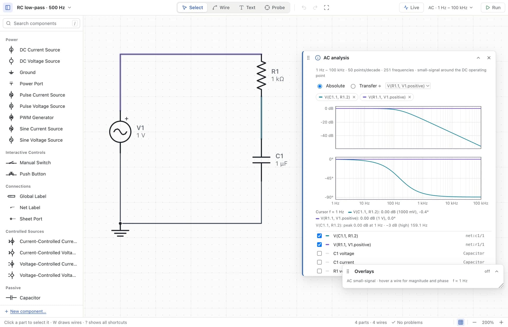
One resistor. One capacitor. Two questions.

Put a 1 kΩ resistor between a source and an output node, then a 1 µF capacitor from that node to ground. This is a first-order low-pass filter when the output is measured across the capacitor. The resistor limits how quickly the source can change the capacitor’s stored charge. Slow changes pass with little attenuation; fast changes are reduced.

A transient asks what voltage appears at each instant. An AC sweep asks how a small sinusoidal perturbation is scaled and shifted at each frequency. For this linear RC circuit, the two views should agree once the transient has settled. They are different analyses, not two plotting styles for the same data.

τ = RC = 1 ms fc = 1 / (2πRC) ≈ 159.15 Hz

First, watch a sine wave pass through it.

Open rc-sine-low-pass.circuit.json. Its source is a 1 V peak, 500 Hz sine. Select Transient, use a 20 ms duration and a 10 µs output step, and run. Plot the input and capacitor voltages. Look near the end of the run, rather than at the first cycle: transients start with zero stored energy, which adds a startup response.

At 500 Hz, the steady-state gain is about 0.3033. A 1 V peak input therefore produces roughly 0.303 V peak at the capacitor. The real desktop capture measured 0.303303 V over the settled part of the result. The numerical samples do not necessarily land on the exact mathematical peak, so do not expect every displayed digit to equal the formula.

The output also lags the input by about 72.3 degrees. With a 2 ms input period, that corresponds to about 0.402 ms. Compare corresponding upward zero crossings after startup, rather than comparing an input peak to an output zero crossing.

|H(f)| = 1 / √(1 + (2πfRC)²) phase = −atan(2πfRC)

Then ask the whole frequency question.

Set the input source’s AC magnitude to 1 V. This is separate from its time-domain sine amplitude. Choose AC sweep, with a decade sweep from 1 Hz to 100 kHz and 50 points per decade. Run and select the capacitor voltage. Transfer mode divides an output by the chosen input reference; this makes the plotted gain meaningful even if you later change the source’s AC magnitude.

At low frequency, the gain approaches 1, or 0 dB. At the corner, the magnitude is 1/√2 ≈ 0.707 of its low-frequency value, which is about −3.01 dB, and the phase is −45 degrees. The captured run located the corner at 159.1 Hz. The frequency samples and interpolation determine how many digits of that readout are useful.

Far above the corner, multiplying frequency by ten reduces magnitude by approximately a factor of ten: a −20 dB-per-decade slope. The phase approaches −90 degrees. At 500 Hz the gain is about −10.36 dB, consistent with the 0.3033 amplitude ratio in the transient.

Make a prediction you can test.

Double the capacitor to 2 µF. The time constant doubles to 2 ms and the corner halves to about 79.6 Hz. At the same 500 Hz input, the steady-state output should fall to roughly 0.157 V peak and lag further. Change only that value, rerun both analyses, and compare with your prediction.

Now restore the capacitor and put a resistor across it. The low-frequency gain is no longer 1 because the added resistance loads the output. The effective resistance seen by the capacitor changes too. A formula for an unloaded RC filter cannot be applied unchanged to this new circuit. This is a useful reason to keep the schematic beside the plot.

Know which knob changes which result.

The output step controls the spacing of stored transient samples. The adaptive solver chooses its internal integration steps separately. Making output samples denser can make a cursor or peak reading more useful, but it does not add missing device physics or automatically improve every numerical error.

AC is a small-signal analysis around a DC operating point. For a nonlinear circuit, it describes a local response; it does not reproduce clipping or a large switching waveform. Likewise, a transient screenshot is not proof that a sweep has been performed. Name the analysis, the measured node, the source settings and the settled interval when comparing results.

A real capacitor has tolerance, leakage and parasitics, and a real source has impedance. Those effects only appear when the model includes them. Use the ideal RC result as a clear baseline, then add the effects that matter to your question.