A component symbol is not the whole component.

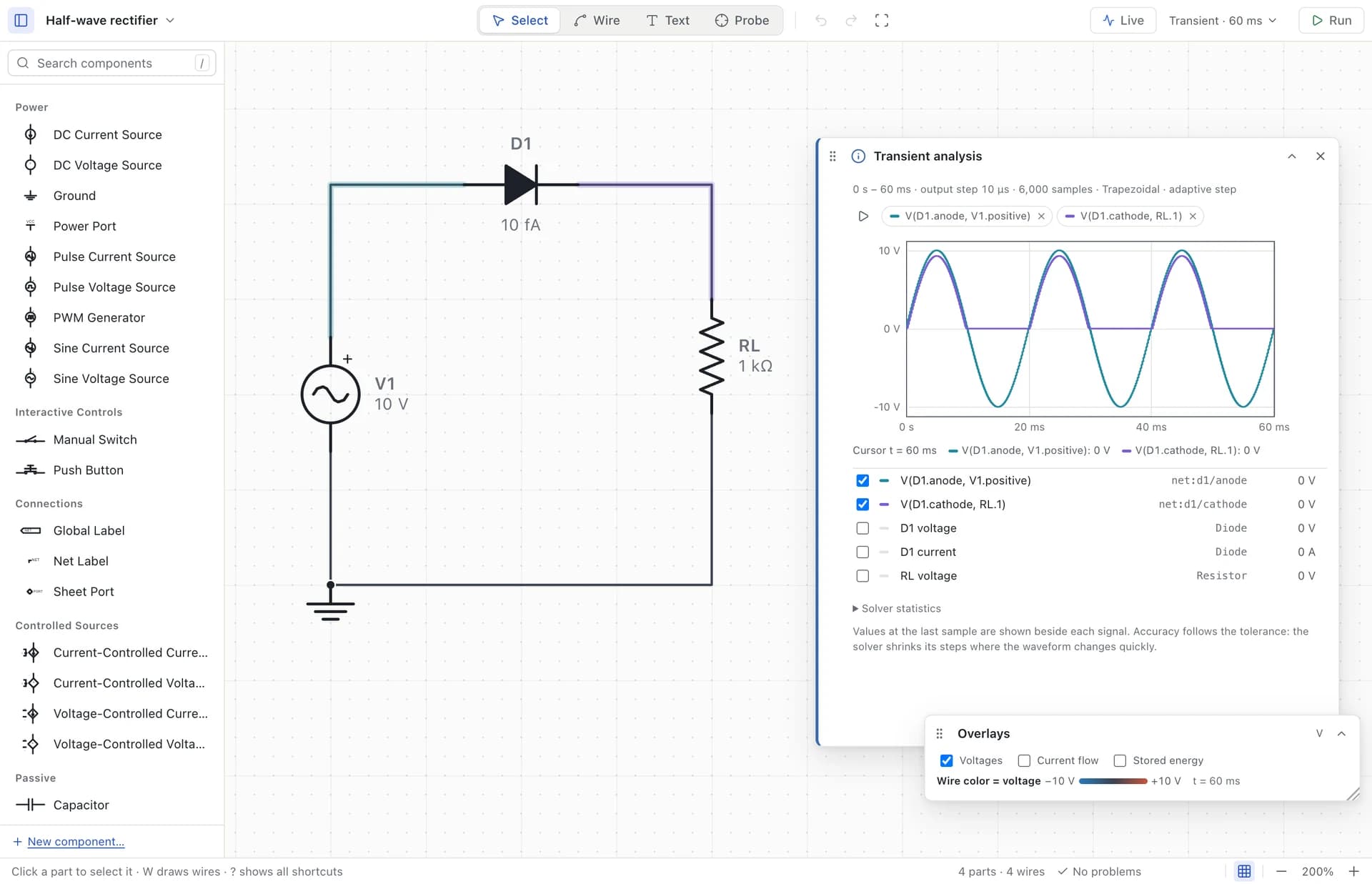
Every result answers a model’s question.

A resistor symbol says little about tolerance, temperature drift or maximum power. A diode symbol says even less about its forward curve, charge storage or thermal behavior. The simulation runs equations and parameters attached to those symbols. A convincing trace tells you what that model does under those conditions, not everything a physical part will do.

This is useful rather than disappointing. A simple model makes cause and effect easier to see. The important habit is to state your question first. If you want to understand why a rectifier passes one half of a sine, a generic diode may be enough. If you want to choose a diode for switching loss at a particular junction temperature, that same model is not sufficient evidence.

Know what the built-in parts represent.

The current desktop uses generic diode and Zener models, with optional junction capacitance and transit time. Those charge-storage parameters default to zero. The forward drop depends on current; a diode is not a universal 0.7 V subtraction. In the half-wave rectifier example, changing the load changes the operating current and can change the forward drop.

Generic BJTs use an Ebers–Moll model; the built-in BJT is static, so it does not represent transistor charge storage. Generic MOSFETs use a Level-1 model with a body diode and optional constant capacitances. A familiar symbol or a successful run does not imply a modern power-device model with all of its nonlinear capacitances and temperature effects.

Transformers and coupled inductors use linear magnetic coupling. Core saturation, loss and winding resistance are not automatically included. Op-amp behavior is also model-dependent; a gain-bandwidth parameter is not a complete datasheet model for slew rate, input limits and transient recovery.

A SPICE file still needs a compatibility check.

Electro can attach supported .MODEL and .SUBCKT definitions and embed their model text in a project. The model compiler distinguishes exact support, a mapped subset and unsupported physics. Read that classification and every warning. A file ending in .lib is not a guarantee that every device or expression in it can run.

For example, supported Level-1 MOS models are not interchangeable with arbitrary BSIM models. Pin mapping matters just as much as the model name: a subcircuit’s declared terminal order must match the symbol’s pins. A plausible output is not evidence that drain and source, or an amplifier’s supply pins, were mapped correctly.

Use a small test bench before putting an imported part into a larger project. Check a few known bias points, signs and operating limits. Keep the model’s source and version with your project notes, and respect its distribution terms when sharing embedded model data. Exporting to another tool also deserves a new warning review; support is not identical in both directions.

Numerical accuracy is a different problem.

Tighter solver tolerances ask for a more accurate solution to the existing equations. They cannot add core saturation to a linear transformer or charge storage to a static transistor. Separate model error from numerical error before spending time on solver settings.

In the current Live controls, Balanced is the normal baseline. Fast loosens local-error tolerances for exploration. Precise is currently equivalent to Balanced and is labelled that way. If a local-error failure offers Retry with Fast accuracy, choosing it explicitly resumes from the saved checkpoint with looser tolerances; it is not proof that the original accuracy target has been met.

For a critical observation, compare runs using different sensible settings and check an analytical case where you can. Watch the sampled interval too: a sparse display can miss a peak, and the Live oscilloscope is a bounded view of the run. More decimal places in a readout are not a calibration certificate.

Build confidence in layers.

A practical workflow keeps each check small enough to explain. You should be able to say which observation supports which conclusion.

1. Start with an analytical case: an unloaded divider, RC time constant or simple current loop. Check units and reference directions.
2. Add one non-ideal effect at a time. Record the model parameters and compare what changed.
3. Check source impedance, load, initial conditions, supply rails and the interval you are measuring. These can dominate the result even with ideal components.
4. For a physical design, compare against the actual datasheet and appropriate measurements. Thermal limits, EMI, protection and component stress need evidence beyond this simulator’s generic models.